Plot a fitted spectrum

This is an example showing how to plot the result of fitting a spectrum using the IBIS8542Model class.

First we shall create a list of wavelengths, with a variable wavelength spacing. Next, we shall use the Voigt profile to generate spectral intensities at each of the wavelength points. Typically you would provide a spectrum obtained from observations.

The data in this example are produced from randomly selected parameters, so numerical values in this example should be ignored.

import numpy as np
from mcalf.models import IBIS8542Model
from mcalf.profiles.voigt import double_voigt

# Create the wavelength grid and intensity values
wavelengths = np.linspace(8541, 8543, 20)
wavelengths = np.delete(wavelengths, np.s_[1:6:2])
wavelengths = np.delete(wavelengths, np.s_[-6::2])

spectrum = double_voigt(wavelengths, -526, 8542, 0.1, 0.1,
                        300, 8541.9, 0.2, 0.05, 1242)

from mcalf.visualisation import plot_spectrum

plot_spectrum(wavelengths, spectrum, normalised=False)

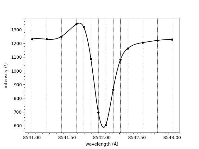
<Axes: xlabel='wavelength (Å)', ylabel='intensity ($I$)'>

A basic model is created,

model = IBIS8542Model(original_wavelengths=wavelengths)

The spectrum is provided to the model’s fit method. A classifier has not been loaded so the classification must be provided manually. The fitting algorithm assumes that the intensity at the ends of the spectrum is zero, so in this case we need to provide it with a background value to subtract from the spectrum before fitting.

fit = model.fit(spectrum=spectrum, classifications=4, background=1242)

print(fit)

Successful FitResult with both profile of classification 4

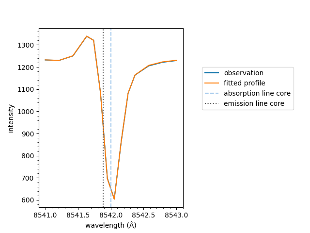
The spectrum can now be plotted,

model.plot(fit, spectrum=spectrum, background=1242)

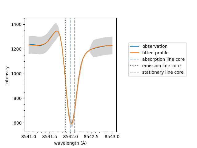
<Axes: xlabel='wavelength (Å)', ylabel='intensity'>

If an array of spectra and associated background values had been loaded into the model with the load_array() and load_background() methods respectively, the spectrum and background parameters would not have to be specified when plotting. This is because the fit object would contain indices that the model object would use to look up the original loaded values.

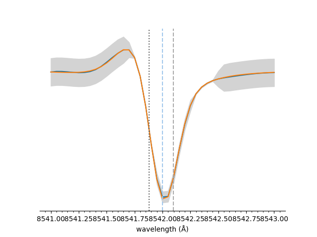
Equivalent to above, the plot method can be called on the fit object directly. Remember to specify the model which is needed for additional information such as the stationary line core value.

fit.plot(model, spectrum=spectrum, background=1242)

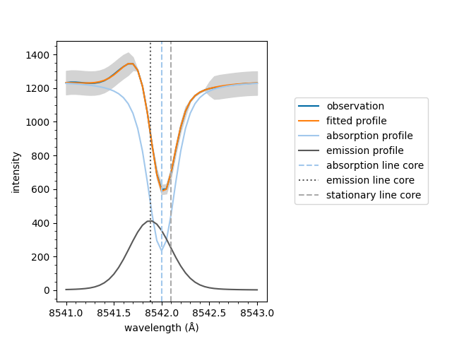
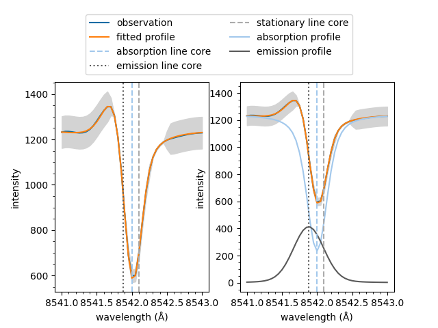
If the fit has multiple spectral components, such as an active emission profile mixed with a quiescent absorption profile, the follow method can be used to plot the components separatly.

If the fit only has a single component the plot method as shown above is used.

model.plot_separate(fit, spectrum=spectrum, background=1242)

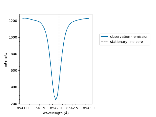
If the fit has an emission component, it is subtracted from the raw spectral data. Otherwise, the default plot method is used.

model.plot_subtraction(fit, spectrum=spectrum, background=1242)

The same line on multiple plots is only labelled the first time it plotted in the figure. This prevents duplicated entries in legends.

import matplotlib.pyplot as plt

fig, ax = plt.subplots(1, 2)

model.plot(fit, spectrum=spectrum, background=1242,
           show_legend=False, ax=ax[0])
model.plot_separate(fit, spectrum=spectrum, background=1242,
                    show_legend=False, ax=ax[1])

fig.subplots_adjust(top=0.75)  # Create space above for legend
fig.legend(ncol=2, loc='upper center', bbox_to_anchor=(0.5, 0.97))

plt.show()

The underlying mcalf.visualisation.plot_ibis8542() function can be used directly. However, it is recommended to plot using the method detailed above as it will do additional processing to the wavelengths and spectrum and also pass additional parameters, such as sigma, to this fitting function.

from mcalf.visualisation import plot_ibis8542

plot_ibis8542(wavelengths, spectrum, fit.parameters, 1242)

<Axes: xlabel='wavelength (Å)', ylabel='intensity'>

The y-axis and legend can be easily hidden,

model.plot(fit, spectrum=spectrum, background=1242,
           show_intensity=False, show_legend=False)

<Axes: xlabel='wavelength (Å)'>