Note
Go to the end to download the full example code
Using IBIS8542Model
This is an example showing how to fit an array of
spectra using the mcalf.models.IBIS8542Model
class, and plot and export the results.
Generate sample data
Create spectral grid
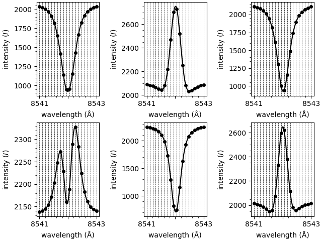
First, we shall generate some random sample data to demonstrate the API. The randomly generated spectra are not intended to be representative of observed spectra numerically, they just have a similar shape.
import numpy as np
import matplotlib.pyplot as plt

from mcalf.profiles.voigt import voigt, double_voigt
from mcalf.visualisation import plot_spectrum

# Create demo wavelength grid
w = np.linspace(8541, 8543, 20)
We shall generate demo spectra in a 2x3 grid. Half of the spectra will have one spectral component (absorption only) and the other half will have two spectral components (mixed absorption and emission components).
Demo spectral components will be modelled as Voigt functions with randomly generated parameters, each within a set range of values.
def v(classification, w, *args):
    """Voigt function wrapper."""
    if classification < 1.5:  # absorption only
        return voigt(w, *args[:4], args[-1])
    return double_voigt(w, *args)  # absorption + emission


def s():
    """Generate random spectra for a 2x3 grid."""
    np.random.seed(0)  # same spectra every time
    p = np.random.rand(9, 6)  # random Voigt parameters
    # 0  1  2  3  4  5  6  7  8  # p index
    # a1 b1 s1 g1 a2 b2 s2 g2 d  # Voigt parameter
    # absorption |emission   |background

    p[0] = 100 * p[0] - 1000  # absorption amplitude
    p[4] = 100 * p[4] + 1000  # emission amplitude

    for i in (1, 5):  # abs. and emi. peak positions
        p[i] = 0.05 * p[i] - 0.025 + 8542

    for i in (2, 3, 6, 7):  # Voigt sigmas and gammas
        p[i] = 0.1 * p[i] + 0.1

    p[8] = 300 * p[8] + 2000  # intensity background constant

    # Define each spectrum's classification
    c = [0, 2, 0, 2, 0, 2]
    # Choose single or double component spectrum
    # based on this inside the function `v()`.

    # Generate the spectra
    specs = [v(c[i], w, *p[:, i]) for i in range(6)]

    # Reshape to 2x3 grid
    return np.asarray(specs).reshape((2, 3, len(w)))


raw_data = s()

print('shape of spectral grid:', raw_data.shape)
shape of spectral grid: (2, 3, 20)
These spectra look as follows,
Compute the background intensity
MCALF does not model a constant background value, i.e., the fitting process assumes the intensity values far out in the spectrum’s wings are zero.
You can however tell MCALF what the constant background value is, and it will subtract it from the spectrum before fitting.
This process was not made automatic as we wanted to give the user full control on setting the background value.
For these demo data, we shall simply set the background
to the first intensity value of every spectrum.
For a real dataset, you may wish to average the
background value throughout a range of spectral points,
or even do a moving average throughout time.
Functions are provided in mcalf.utils.smooth to
assist with this process.
backgrounds = raw_data[:, :, 0]

print('shape of background intensity grid:', backgrounds.shape)
shape of background intensity grid: (2, 3)
Define a demo classifier
In this example we will not demonstrate how to create
a neural network classifier. MCALF offers a lot of
flexibility when it comes to the classifier. This
demo classifier outlines the basic API that is
required. By default, the model has a
sklearn.neural_network.MLPClassifier
object preloaded for use as the classifier.
The methods mcalf.models.ModelBase.train()
and mcalf.models.ModelBase.test() are
provided by MCALF to assist with training the
neural network. There is also a useful script
in the Getting Started section under
User Documentation in the sidebar for
semi-automating the process of creating the
ground truth dataset.
Please see tutorials for packages such as scikit-learn for more in-depth advice on creating classifiers.
As we only have six spectra with two distinct shapes, we can create a very simple classifier that classifies spectra based on whether their central intensity is greater or smaller than the left most intensity.
class DemoClassifier:
    @staticmethod
    def predict(X):
        y = np.zeros(len(X), dtype=int)
        y[X[:, len(X[0]) // 2] > X[:, 0]] = 2
        return y
Using IBIS8542Model with the generated data
Initialise the model
Everything we have been doing up to this point has been creating the demo data and classifier. Now we can actually create a model and load in the demo data, although the following steps would be identical for a real dataset.
from mcalf.models import IBIS8542Model

# Initialise the model with the wavelength grid
model = IBIS8542Model(original_wavelengths=w)

# Load the spectral shape classifier
model.neural_network = DemoClassifier

# Load the array of spectra and background intensities
model.load_array(raw_data, ['row', 'column', 'wavelength'])
model.load_background(backgrounds, ['row', 'column'])
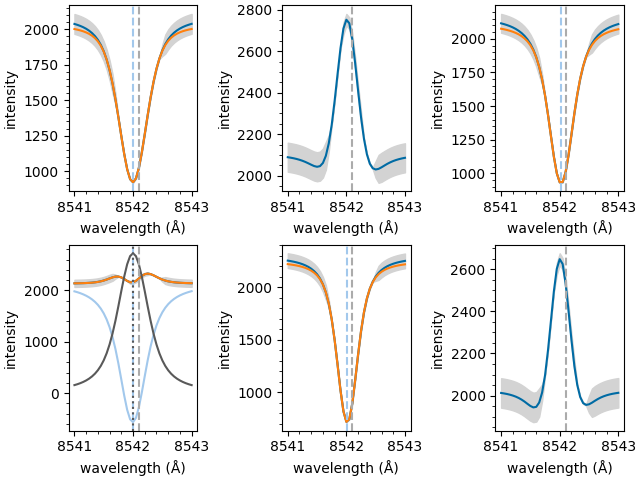
Fit the loaded data
We have now fully initialised the model. We can now
call methods to fit the model to the loaded spectra.
In the following step we fit all the loaded spectra
and a 1D list of FitResult
objects is returned.
Processing 6 spectra
/home/docs/checkouts/readthedocs.org/user_builds/mcalf/checkouts/stable/src/mcalf/models/base.py:1003: UserWarning: RuntimeError(Optimal parameters not found: The maximum number of function evaluations is exceeded.) at (0, 0, 1)
  warnings.warn(f"RuntimeError({e}){location_text}")
/home/docs/checkouts/readthedocs.org/user_builds/mcalf/checkouts/stable/src/mcalf/models/base.py:1003: UserWarning: RuntimeError(Optimal parameters not found: The maximum number of function evaluations is exceeded.) at (0, 1, 2)
  warnings.warn(f"RuntimeError({e}){location_text}")
[Successful FitResult with absorption profile of classification 0, Unsuccessful FitResult with both profile of classification 2, Successful FitResult with absorption profile of classification 0, Successful FitResult with both profile of classification 2, Successful FitResult with absorption profile of classification 0, Unsuccessful FitResult with both profile of classification 2]
Plot the fitted parameters
The individual components of each fit can now be plotted separately,
Extract processed spectra
As well as fitting spectra, we can call other methods. In this step we’ll extract the array of loaded spectra. However, these spectra have been re-interpolated to a new finer wavelength grid. (This grid can be customised when initialising the model.)
spectra = model.get_spectra(row=[0, 1], column=range(3))

print('new shape of spectral grid:', spectra.shape)

spectra_1d = spectra.reshape((6, spectra.shape[-1]))

fig, axes = plt.subplots(2, 3, constrained_layout=True)
for ax, spec in zip(axes.flat, spectra_1d):

    plot_spectrum(model.constant_wavelengths, spec,
                  normalised=False, ax=ax)

plt.show()
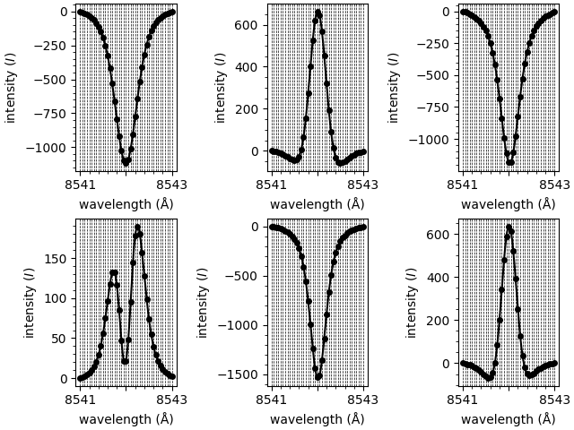
new shape of spectral grid: (1, 2, 3, 41)
Classify spectra
We can also classify the loaded spectra and create plots,
classifications = model.classify_spectra(row=[0, 1], column=range(3))

print('classifications are:', classifications)
classifications are: [[[0 2 0]
  [2 0 2]]]
This function plots the spectra grouped by classification,
from mcalf.visualisation import plot_classifications

plot_classifications(spectra_1d, classifications.flatten())
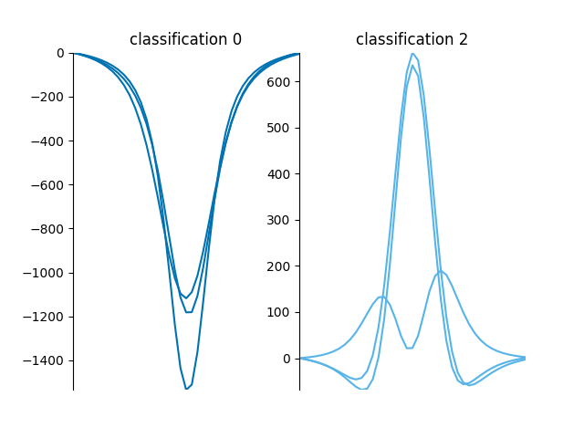
GridSpec(1, 2)
This function plots a spatial map of the classifications on the 2x3 grid,
from mcalf.visualisation import plot_class_map

plot_class_map(classifications)
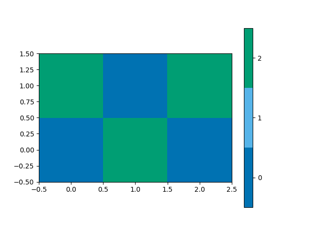
<matplotlib.image.AxesImage object at 0x7f0cc53bb6d0>
Merge output data
The FitResult objects in the
fits 1D list can be merged into a grid.
Each of these objects can be appended to a
single FitResults object.
This allows for increased data portability,
from mcalf.models import FitResults

# Initialise with the grid shape and num. params.
results = FitResults((2, 3), 8)

# Append each fit to the object
for fit in fits:
    results.append(fit)
Now that we have appended all 6 fits, we can access the merged data,
print(results.classifications)
print(results.profile)
print(results.success)
print(results.parameters)
[[0 2 0]
 [2 0 2]]
[['absorption' 'both' 'absorption']
 ['both' 'absorption' 'both']]
[[ True False  True]
 [ True  True False]]
[[[-8.12854071e+02  8.54199697e+03  1.78499712e-01  1.26560705e-01
               nan             nan             nan             nan]
  [            nan             nan             nan             nan
               nan             nan             nan             nan]
  [-8.18417945e+02  8.54202321e+03  1.28952238e-01  1.56493579e-01
               nan             nan             nan             nan]]

 [[-2.21478736e+03  8.54199483e+03  1.06846047e-01  2.21738766e-01
    2.33701044e+03  8.54199968e+03  1.48605642e-01  2.05127799e-01]
  [-8.73401645e+02  8.54201460e+03  1.15790594e-01  1.20586703e-01
               nan             nan             nan             nan]
  [            nan             nan             nan             nan
               nan             nan             nan             nan]]]
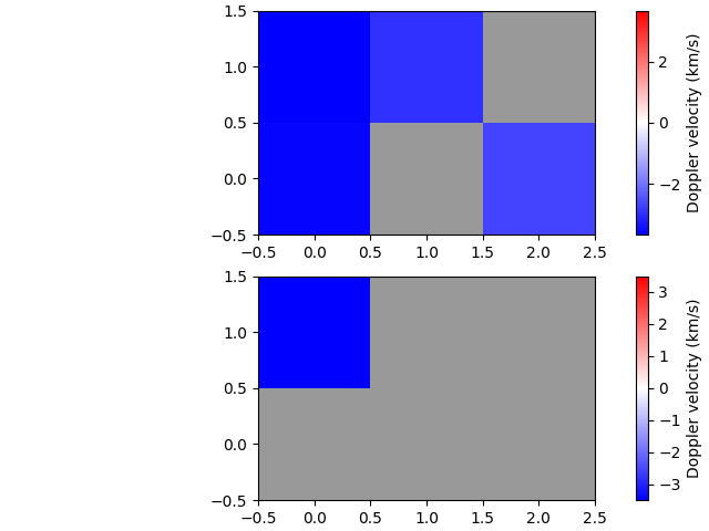
Calculate velocities
And finally, we can calculate Doppler velocities for both the quiescent (absorption) and active (emission) regimes. (The model needs to be given so the stationary line core wavelength is available.)
Export to FITS file
The FitResults object can
also be exported to a FITS file,
results.save('ibis8542model_demo_fit.fits', model)
The file has the following structure,
Filename: ibis8542model_demo_fit.fits
No.    Name      Ver    Type      Cards   Dimensions   Format
  0  PRIMARY       1 PrimaryHDU      13   (0,)
  1  PARAMETERS    1 ImageHDU        12   (8, 3, 2)   float64
  2  CLASSIFICATIONS    1 ImageHDU        10   (3, 2)   int16
  3  PROFILE       1 ImageHDU        11   (3, 2)   int16
  4  SUCCESS       1 ImageHDU        10   (3, 2)   int16
  5  CHI2          1 ImageHDU        10   (3, 2)   float64
  6  VLOSA         1 ImageHDU        12   (3, 2)   float64
  7  VLOSQ         1 ImageHDU        12   (3, 2)   float64
This example outlines the basics of using the
mcalf.models.IBIS8542Model class.
Typically millions of spectra would need to be
fitted and processed at the same time.
For more details on running big jobs and how
spectra can be fitted in parallel, see
the Working with IBIS data example in the
gallery.
Note
Due to limitations with the documentation hosting provider, the examples in the MCALF documentation are computed using a Python based implementation of the Voigt profile instead of the more efficient C version. When this code is run on your own machine it should take much less time than the value reported below.
Total running time of the script: ( 0 minutes 6.928 seconds)