Working with IBIS data

This example shows how to initialise the mcalf.models.IBIS8542Model class with real IBIS data, and train a neural network classifier. We then proceed to fit the array of spectra and visualise the results.

Download sample data

First, the sample data needs to be downloaded from the GitHub repository where it is hosted. This will create four new files in the current directory (about 651 KB total). You may need to install the requests Python package for this step to run.

import requests

path = 'https://raw.githubusercontent.com/ConorMacBride/mcalf/main/examples/data/ibis8542data/'

for file in ('wavelengths.txt', 'spectra.fits',
             'training_data.json', 'results.fits'):
    r = requests.get(path + file, allow_redirects=True)
    with open(file, 'wb') as f:
        f.write(r.content)

Load the sample data

Next, the downloaded data needs to be loaded into Python.

# Import the packages needed for loading data
import json
import numpy as np
from astropy.io import fits

# Load the spectra's wavelength points
wavelengths = np.loadtxt('wavelengths.txt', dtype='>f4')

# Load the array of spectra
with fits.open('spectra.fits') as hdul:
    spectra = hdul[0].data

# Load indices of labelled spectra
with open('training_data.json', 'r') as f:
    data = f.read()
training_data = json.loads(data)

As you can see, the sample data consists of a 60 by 50 array of spectra with 27 wavelength points,

print(wavelengths.shape, spectra.shape)

(27,) (27, 60, 50)

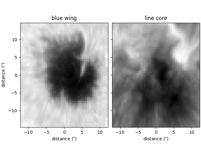
The blue wing and line core intensity values of the spectra are plotted below for illustrative purposes,

import matplotlib.pyplot as plt
import astropy.units as u
from mcalf.visualisation import plot_map

fig, ax = plt.subplots(1, 2, sharey=True, constrained_layout=True)

wing_data = np.log(spectra[0])
core_data = np.log(spectra[len(wavelengths)//2])

res = {
    'offset': (-25, -30),
    'resolution': (0.098 * 5 * u.arcsec, 0.098 * 5 * u.arcsec),
    'show_colorbar': False,
}

wing = plot_map(wing_data, ax=ax[0], **res,
                vmin=np.min(wing_data), vmax=np.max(wing_data))
core = plot_map(core_data, ax=ax[1], **res,
                vmin=np.min(core_data), vmax=np.max(core_data))

wing.set_cmap('gray')
core.set_cmap('gray')

ax[0].set_title('blue wing')
ax[1].set_title('line core')
ax[1].set_ylabel('')

plt.show()

Generate the backgrounds array

As discussed in the Using IBIS8542Model example, a background intensity value must be specified for each spectrum.

For this small sample dataset, we shall simply use the average of the four leftmost intensity values of each spectrum,

backgrounds = np.mean(spectra[:4], axis=0)

Initialise the IBIS8542Model

The loaded data can now be passed into an mcalf.models.IBIS8542Model object.

import mcalf.models

model = mcalf.models.IBIS8542Model(original_wavelengths=wavelengths, random_state=0)

model.load_background(backgrounds, ['row', 'column'])
model.load_array(spectra, ['wavelength', 'row', 'column'])

Training the neural network

By default, the mcalf.models.IBIS8542Model object is loaded with an untrained neural network,

model.neural_network

GridSearchCV(cv=5,
             estimator=MLPClassifier(hidden_layer_sizes=(40,), max_iter=1000,
                                     random_state=0, solver='lbfgs'),
             n_jobs=-1,
             param_grid={'alpha': [1e-05, 2e-05, 3e-05, 4e-05, 5e-05, 6e-05,
                                   7e-05, 8e-05, 9e-05]})

In a Jupyter environment, please rerun this cell to show the HTML representation or trust the notebook.
On GitHub, the HTML representation is unable to render, please try loading this page with nbviewer.org.

The mcalf.models.IBIS8542Model class provides two methods to train and test the loaded neural network.

The training_data.json file contains a dictionary of indices for each classification 0 to 5. These indices correspond to randomly pre-chosen spectra in the spectra.fits file.

The training set consists of 200 spectra; 40 for each classification. This training set is for demonstration purposes only, generally it is not recommended to train with such a relatively high percentage of your data, as the risk of overfitting the neural network to this specific 60 by 50 array is increased.

To begin, we’ll convert the list of indices into a list of spectra and corresponding classifications,

from mcalf.utils.spec import normalise_spectrum


def select_training_set(indices, model):
    for c in sorted([int(i) for i in indices.keys()]):
        i = indices[str(c)]
        spectra = np.array([normalise_spectrum(
            model.get_spectra(row=j, column=k)[0, 0, 0],
            model.constant_wavelengths, model.constant_wavelengths
        ) for j, k in i])
        try:
            _X = np.vstack((_X, spectra))
            _y = np.hstack((_y, [c] * len(spectra)))
        except NameError:
            _X = spectra
            _y = [c] * len(spectra)
    return _X, _y


X, y = select_training_set(training_data, model)

print(X.shape)  # spectra
print(y.shape)  # labels/classifications

(200, 49)
(200,)

These classifications look as follows,

from mcalf.visualisation import plot_classifications

plot_classifications(X, y)

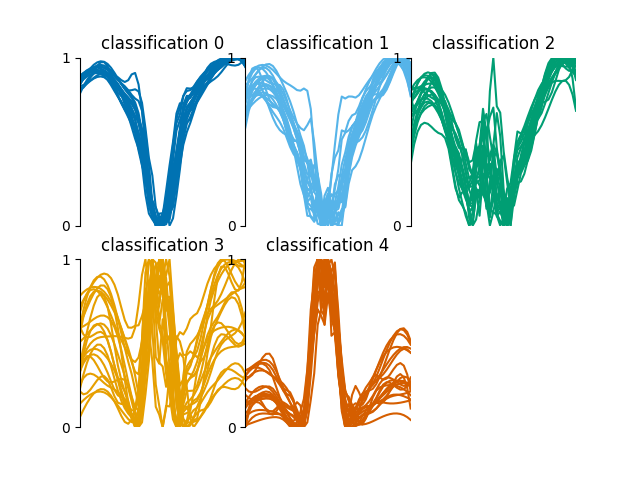
GridSpec(2, 3)

Now we can train the neural network on 100 labelled spectra (even indices),

model.train(X[::2], y[::2])

And now we can use the other 100 labelled spectra (odd indices) to test the performance of the neural network,

model.test(X[1::2], y[1::2])

+---------------------------------------------+
|      Neural Network Testing Statistics      |
+---------------------------------------------+
| Percentage predictions==labels ::  89.00%   |
+---------------------------------------------+
| Average deviation for each classification   |
+---------------------------------------------+
|     class  0 ::   0.00 ±  0.00              |
+---------------------------------------------+
|     class  1 ::   0.20 ±  0.68              |
+---------------------------------------------+
|     class  2 ::   0.10 ±  0.44              |
+---------------------------------------------+
|     class  3 ::   0.00 ±  0.32              |
+---------------------------------------------+
|     class  4 ::  -0.05 ±  0.22              |
+---------------------------------------------+
| Average deviation overall ::   0.05 ±  0.41 |
+---------------------------------------------+
              precision    recall  f1-score   support

           0       0.95      1.00      0.98        20
           1       0.94      0.80      0.86        20
           2       0.89      0.80      0.84        20
           3       0.75      0.90      0.82        20
           4       0.95      0.95      0.95        20

    accuracy                           0.89       100
   macro avg       0.90      0.89      0.89       100
weighted avg       0.90      0.89      0.89       100

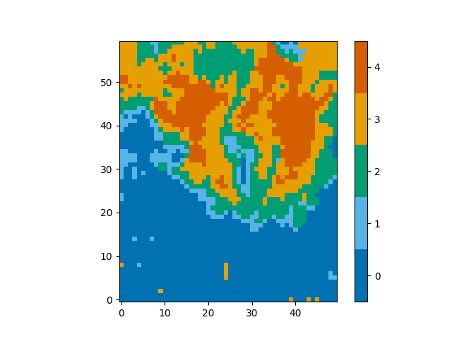
Now that we have a trained neural network, we can use it to classify spectra. Usually spectra will be classified automatically during the fitting process, however, you can request the classification by themselves,

classifications = model.classify_spectra(row=range(60), column=range(50))

These classifications look as follows,

from mcalf.visualisation import plot_class_map

plot_class_map(classifications)

<matplotlib.image.AxesImage object at 0x7f7b5eadc430>

Creating a reproducible classifier

The neural network classifier introduces a certain amount of randomness when it it fitting based on the training data. This randomness arises in the initial values of the weights and biases that are fitted during the training process, as well as the order in which the training data are used.

This means that two neural networks trained on identical data will not produce the same results. To aid the reproducibility of results that rely on a neural network’s classifications, a random_state integer can be passed to mcalf.models.IBIS8542Model as we did above. When we set this value to an integer, no matter how many times we train the neural network on the same data, it will always give the same results.

Until better solutions are available to store trained neural networks, a trained neural network can be saved to a Python pickle file and later reloaded. For maximum compatibility, it is recommended to reload into the same version of scikit-learn and its dependencies.

The neural network trained above can be saved as follows,

import pickle
pkl = open('trained_neural_network.pkl', 'wb')
pickle.dump(model.neural_network, pkl)
pkl.close()

This trained neural network can then be reloaded at a later date as follows,

import pickle
pkl = open('trained_neural_network.pkl', 'rb')
model.neural_network = pickle.load(pkl)  # Overwrite the default untrained model

And you can see that the classifications of spectra are the same,

plot_class_map(model.classify_spectra(row=range(60), column=range(50)))

<matplotlib.image.AxesImage object at 0x7f7b3fd73f10>

Please see the scikit-learn documentation for more details on model persistence.

Fitting the spectra

Now that the data have been loaded and the neural network has been trained, we can proceed to fit the spectra.

Using pre-calculated results

As our 60 by 50 array contains 3000 spectra, it would take roughly 10 minutes to fit them all over 6 processing pools. We include pre-calculated results in the downloaded results.fits file.

The next step of the example loads this file back into Python as though we have just directly calculated it. This isn’t something you would usually need to do, so do not worry about the contents of the load_results() function, however, we plan to include this functionality in MCALF itself in the future.

def load_results(file):

    with fits.open(file) as hdul:
        for hdu in hdul:
            if hdu.name == 'PARAMETERS':
                r_parameters = hdu.data.copy().reshape(-1, 8)
            elif hdu.name == 'CLASSIFICATIONS':
                r_classifications = hdu.data.copy().flatten()
                r_profile = np.full_like(r_classifications, 'both', dtype=object)
                r_profile[r_classifications <= 1] = 'absorption'
            elif hdu.name == 'SUCCESS':
                r_success = hdu.data.copy().flatten()
            elif hdu.name == 'CHI2':
                r_chi2 = hdu.data.copy().flatten()

    results = []
    for i in range(len(r_parameters)):
        fitted_parameters = r_parameters[i]
        fit_info = {
            'classification': r_classifications[i],
            'profile': r_profile[i],
            'success': r_success[i],
            'chi2': r_chi2[i],
            'index': [0, *np.unravel_index(i, (60, 50))],
        }
        if fit_info['profile'] == 'absorption':
            fitted_parameters = fitted_parameters[:4]
        results.append(mcalf.models.FitResult(fitted_parameters, fit_info))

    return results


result_list = load_results('results.fits')

result_list[:4]  # The first four

[Successful FitResult at (0, 0, 0) with absorption profile of classification 0, Successful FitResult at (0, 0, 1) with absorption profile of classification 0, Successful FitResult at (0, 0, 2) with absorption profile of classification 0, Successful FitResult at (0, 0, 3) with absorption profile of classification 0]

Using your own results

You can run the following code to generate the result_list variable for yourself. Try starting with a smaller range of rows and columns, and set the number of pools based on the specification of your processor.

# result_list = model.fit(row=range(60), column=range(50), n_pools=6)

The order of the mcalf.models.FitResult objects in this list will also differ as the order that spectra finish fitting in each pool is unpredictable.

Merging the FitResult objects

The list of mcalf.models.FitResult objects can be mergerd into a mcalf.models.FitResults object, and then saved to a file, just like the results.fits file downloaded earlier.

First the object needs to be initialised with the spatial dimensions and number of fitted parameters,

results = mcalf.models.FitResults((60, 50), 8)

Now we can loop through the list of fits and append them to this object,

for fit in result_list:
    results.append(fit)

This object can then be saved to file,

results.save('ibis8542data.fits', model)

The file has the following structure,

with fits.open('ibis8542data.fits') as hdul:
    hdul.info()

Filename: ibis8542data.fits
No.    Name      Ver    Type      Cards   Dimensions   Format
  0  PRIMARY       1 PrimaryHDU      13   (0,)
  1  PARAMETERS    1 ImageHDU        12   (8, 50, 60)   float64
  2  CLASSIFICATIONS    1 ImageHDU        10   (50, 60)   int16
  3  PROFILE       1 ImageHDU        11   (50, 60)   int16
  4  SUCCESS       1 ImageHDU        10   (50, 60)   int16
  5  CHI2          1 ImageHDU        10   (50, 60)   float64
  6  VLOSA         1 ImageHDU        12   (50, 60)   float64
  7  VLOSQ         1 ImageHDU        12   (50, 60)   float64

Exploring the fitted data

You can plot a fitted spectrum as follows,

model.plot(result_list[0])

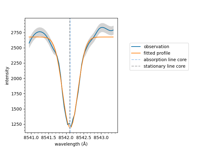
<Axes: xlabel='wavelength (Å)', ylabel='intensity'>

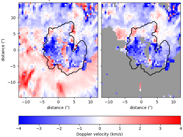
You can calculate and plot Doppler velocities for both the quiescent and active regimes as follows, (with an outline of the sunspot’s umbra),

vq = results.velocities(model, vtype='quiescent')
va = results.velocities(model, vtype='active')

umbra_mask = np.full_like(backgrounds, True)
umbra_mask[backgrounds < 1100] = False

fig, ax = plt.subplots(1, 2, sharey=True, constrained_layout=True)

settings = {
    'show_colorbar': False, 'vmax': 4, 'offset': (-25, -30),
    'resolution': (0.098 * 5 * u.arcsec, 0.098 * 5 * u.arcsec),
    'umbra_mask': umbra_mask,
}

im = plot_map(vq, ax=ax[0], **settings)
plot_map(va, ax=ax[1], **settings)

ax[0].set_title('quiescent')
ax[1].set_title('active')
ax[1].set_ylabel('')
fig.colorbar(im, ax=ax, location='bottom', label='Doppler velocity (km/s)')

plt.show()